In the last part of the data science tutorial, we saw how to establish the correlation between the typical parameters of a FDM 3D printing machine i.e., layer height, nozzle temperature, material etc. and the printed part quality parameters i.e., strength, elongation etc.
In this part we will see how to actually build different machine learning models for the prediction of the additive manufactured part quality. We will also see how the different ML models compare interns of accuracy and over-fitting.
If you remember, the dataset have the following features:
layer_height
wall_thickness
infill_density
infill_pattern
nozzle_temperature
bed_temperature
print_speed
material
fan_speed
roughness
tension_strenght
elongation
And the first few instances of our dataset looks like this:
| layer_height | wall_thickness | infill_density | infill_pattern | nozzle_temperature | bed_temperature | print_speed | material | fan_speed | roughness | tension_strenght | elongation | |
|---|---|---|---|---|---|---|---|---|---|---|---|---|
| 0 | 0.02 | 8 | 90 | grid | 220 | 60 | 40 | abs | 0 | 25 | 18 | 1.2 |
| 1 | 0.02 | 7 | 90 | honeycomb | 225 | 65 | 40 | abs | 25 | 32 | 16 | 1.4 |
| 2 | 0.02 | 1 | 80 | grid | 230 | 70 | 40 | abs | 50 | 40 | 8 | 0.8 |
| 3 | 0.02 | 4 | 70 | honeycomb | 240 | 75 | 40 | abs | 75 | 68 | 10 | 0.5 |
| 4 | 0.02 | 6 | 90 | grid | 250 | 80 | 40 | abs | 100 | 92 | 5 | 0.7 |
Out of these the infill_pattern and material are categorical in nature, which we need to encode to the numerical data:
#converting text labels to numbers
from sklearn.preprocessing import LabelEncoder
labelencoder = LabelEncoder()
df['infill_pattern'] = labelencoder.fit_transform(df['infill_pattern'])

labelencoder1 = LabelEncoder()
df['material'] = labelencoder1.fit_transform(df['material'])
Now if we check the dataset, it looks like:
| layer_height | wall_thickness | infill_density | infill_pattern | nozzle_temperature | bed_temperature | print_speed | material | fan_speed | roughness | tension_strenght | elongation | |
|---|---|---|---|---|---|---|---|---|---|---|---|---|
| 0 | 0.02 | 8 | 90 | 0 | 220 | 60 | 40 | 0 | 0 | 25 | 18 | 1.2 |
| 1 | 0.02 | 7 | 90 | 1 | 225 | 65 | 40 | 0 | 25 | 32 | 16 | 1.4 |
| 2 | 0.02 | 1 | 80 | 0 | 230 | 70 | 40 | 0 | 50 | 40 | 8 | 0.8 |
| 3 | 0.02 | 4 | 70 | 1 | 240 | 75 | 40 | 0 | 75 | 68 | 10 | 0.5 |
| 4 | 0.02 | 6 | 90 | 0 | 250 | 80 | 40 | 0 | 100 | 92 | 5 | 0.7 |
Please observe the change in the values of the two categorical features.
We now want to normalize the non-categorical features:
#selecting all the columns except the ones with catagorical values
df1=df[df.columns.difference(["infill_pattern", "material"])]

normalized_df=(df1-df1.min())/(df1.max()-df1.min())
Joining the normalized non-categorical features and the encoded categorical features:
#selecting all the columns except the ones with catagorical values
df1=df[df.columns.difference(["infill_pattern", "material"])]
The dataset , now, looks like:
n_df1.head()| bed_temperature | elongation | fan_speed | infill_density | layer_height | nozzle_temperature | print_speed | roughness | tension_strenght | wall_thickness | |
|---|---|---|---|---|---|---|---|---|---|---|
| 0 | 60 | 1.2 | 0 | 90 | 0.02 | 220 | 40 | 25 | 18 | 8 |
| 1 | 65 | 1.4 | 25 | 90 | 0.02 | 225 | 40 | 32 | 16 | 7 |
| 2 | 70 | 0.8 | 50 | 80 | 0.02 | 230 | 40 | 40 | 8 | 1 |
| 3 | 75 | 0.5 | 75 | 70 | 0.02 | 240 | 40 | 68 | 10 | 4 |
| 4 | 80 | 0.7 | 100 | 90 | 0.02 | 250 | 40 | 92 | 5 | 6 |
n_df1_test_train=n_df1In this dataset, there are three target variables (roughness, tensile_strength, elongation). To keep the things simple we are not going to use Multi Target Regression (MTR) , rather we will separate the three targets and run regression separately:
y1=n_df1_test_train[['roughness']]
y2=n_df1_test_train[['tension_strenght']]
y3=n_df1_test_train[['elongation']]
X=n_df1_test_train[n_df1_test_train.columns.difference(['roughness', 'tension_strenght', 'elongation'])]
We need to split the dataset between test and train:
from sklearn.model_selection import train_test_split
#X_train, X_test, y_train, y_test = train_test_split(X, y, test_size=0.33, random_state=42)
X1_train, X1_test, y1_train, y1_test = train_test_split(X, y1, test_size=0.5, random_state=42)
X2_train, X2_test, y2_train, y2_test = train_test_split(X, y2, test_size=0.33, random_state=42)
X3_train, X3_test, y3_train, y3_test = train_test_split(X, y3, test_size=0.33, random_state=42)
We then will use the spitted dataset to build different machine learning models (Linear regression, polynomial regression, MLP regression, KNN regression, Ridge regression). Will train each of the models for the train dataset split, and calculate the accuracy using the test dataset:
#linear regression
from sklearn.linear_model import LinearRegression
linreg = LinearRegression().fit(X1_train, y1_train)
print('R-squared score X1-roughness(training): {:.3f}'
.format(linreg.score(X1_train, y1_train)))
print('R-squared score X1-roughness(test): {:.3f}'
.format(linreg.score(X1_test, y1_test)))
R-squared score X1-roughness(training): 0.907
R-squared score X1-roughness(test): 0.746
from sklearn.linear_model import LinearRegression
linreg2 = LinearRegression().fit(X2_train, y2_train)
print('R-squared score X2-tension_strength(training): {:.3f}'
.format(linreg2.score(X2_train, y2_train)))
print('R-squared score X2-tension_strength(test): {:.3f}'
.format(linreg2.score(X2_test, y2_test)))
R-squared score X2-tension_strength(training): 0.652
R-squared score X2-tension_strength(test): 0.662
from sklearn.linear_model import LinearRegression
linreg3 = LinearRegression().fit(X3_train, y3_train)
print('R-squared score X3-elongation(training): {:.3f}'
.format(linreg3.score(X3_train, y3_train)))
print('R-squared score X3-elongation(test): {:.3f}'
.format(linreg3.score(X3_test, y3_test)))
R-squared score X3-elongation(training): 0.718
R-squared score X3-elongation(test): 0.663
# Fitting Polynomial Regression to the dataset
from sklearn.preprocessing import PolynomialFeatures
poly = PolynomialFeatures(degree = 4)
X1_train_poly = poly.fit_transform(X1_train)
X1_test_poly = poly.fit_transform(X1_test)
poly.fit(X1_train_poly, y1_train)
lin2 = LinearRegression()
lin2.fit(X1_train_poly, y1_train)
print('R-squared score X1_poly-roughness(training): {:.3f}'
.format(lin2.score(X1_train_poly, y1_train)))
print('R-squared score X1_poly-roughness(test): {:.3f}'
.format(lin2.score(X1_test_poly, y1_test)))
R-squared score X1_poly(training): 1.000
R-squared score X1_poly(test): 0.619
# Fitting Polynomial Regression to the dataset
from sklearn.preprocessing import PolynomialFeatures
poly = PolynomialFeatures(degree = 4)
X2_train_poly = poly.fit_transform(X2_train)
X2_test_poly = poly.fit_transform(X2_test)
poly.fit(X2_train_poly, y2_train)
lin2_2 = LinearRegression()
lin2_2.fit(X2_train_poly, y2_train)
print('R-squared score X2_poly-tensileStrength(training): {:.3f}'
.format(lin2_2.score(X2_train_poly, y2_train)))
print('R-squared score X2_poly-tensileStrength(test): {:.3f}'
.format(lin2_2.score(X2_test_poly, y2_test)))
R-squared score X2_poly-tensileStrength(training): 1.000
R-squared score X2_poly-tensileStrength(test): -0.713
# Fitting Polynomial Regression to the dataset
from sklearn.preprocessing import PolynomialFeatures
poly = PolynomialFeatures(degree = 4)
X3_train_poly = poly.fit_transform(X3_train)
X3_test_poly = poly.fit_transform(X3_test)
poly.fit(X3_train_poly, y3_train)
lin2_3 = LinearRegression()
lin2_3.fit(X3_train_poly, y3_train)
print('R-squared score X3_poly-elongation(training): {:.3f}'
.format(lin2_3.score(X3_train_poly, y3_train)))
print('R-squared score X3_poly-elongation(test): {:.3f}'
.format(lin2_3.score(X3_test_poly, y3_test)))
R-squared score X3_poly-elongation(training): 1.000
R-squared score X3_poly-elongation(test): 0.395
#nural net
from sklearn.neural_network import MLPRegressor
#mlpreg = MLPRegressor(hidden_layer_sizes = [100,100],activation = 'tanh',alpha = 0.0003,solver = 'lbfgs').fit(X1_train, y1_train)
mlpreg = MLPRegressor(hidden_layer_sizes = [100,100],activation = 'relu',alpha = 0.0003,solver = 'lbfgs').fit(X1_train, y1_train)
print('R-squared score X1_nn(training): {:.3f}'
.format(mlpreg.score(X1_train, y1_train)))
print('R-squared score X1_nn(test): {:.3f}'
.format(mlpreg.score(X1_test, y1_test)))
R-squared score X1_nn(training): 1.000
R-squared score X1_nn(test): 0.828
#nural net
from sklearn.neural_network import MLPRegressor
#mlpreg = MLPRegressor(hidden_layer_sizes = [100,100],activation = 'tanh',alpha = 0.0003,solver = 'lbfgs').fit(X1_train, y1_train)
mlpreg2 = MLPRegressor(hidden_layer_sizes = [100,100],activation = 'relu',alpha = 0.0003,solver = 'lbfgs').fit(X2_train, y2_train)
print('R-squared score X2_nn-tensileStrength(training): {:.3f}'
.format(mlpreg2.score(X2_train, y2_train)))
print('R-squared score X1_nn-tensileStrength(test): {:.3f}'
.format(mlpreg2.score(X2_test, y2_test)))
/home/suvo/anaconda3/envs/py37/lib/python3.7/site-packages/sklearn/neural_network/multilayer_perceptron.py:1321: DataConversionWarning: A column-vector y was passed when a 1d array was expected. Please change the shape of y to (n_samples, ), for example using ravel().
y = column_or_1d(y, warn=True)
R-squared score X2_nn-tensileStrength(training): 1.000
R-squared score X1_nn-tensileStrength(test): 0.532
#nural net
from sklearn.neural_network import MLPRegressor
#mlpreg = MLPRegressor(hidden_layer_sizes = [100,100],activation = 'tanh',alpha = 0.0003,solver = 'lbfgs').fit(X1_train, y1_train)
mlpreg3 = MLPRegressor(hidden_layer_sizes = [100,100],activation = 'relu',alpha = 0.0003,solver = 'lbfgs').fit(X3_train, y3_train)
print('R-squared score X3_nn-elongation(training): {:.3f}'
.format(mlpreg3.score(X3_train, y3_train)))
print('R-squared score X3_nn-elongation(test): {:.3f}'
.format(mlpreg3.score(X3_test, y3_test)))
/home/suvo/anaconda3/envs/py37/lib/python3.7/site-packages/sklearn/neural_network/multilayer_perceptron.py:1321: DataConversionWarning: A column-vector y was passed when a 1d array was expected. Please change the shape of y to (n_samples, ), for example using ravel().
y = column_or_1d(y, warn=True)
R-squared score X3_nn-elongation(training): 1.000
R-squared score X3_nn-elongation(test): 0.676
#KNN regression
from sklearn.neighbors import KNeighborsRegressor
knnreg = KNeighborsRegressor(n_neighbors = 1).fit(X1_train, y1_train)
print('R-squared score X1_knnreg(training): {:.3f}'
.format(knnreg.score(X1_train, y1_train)))
print('R-squared score X1_knnreg(test): {:.3f}'
.format(knnreg.score(X1_test, y1_test)))
R-squared score X1_knnreg(training): 1.000
R-squared score X1_knnreg(test): -0.150
#KNN regression-X2
from sklearn.neighbors import KNeighborsRegressor
knnreg2 = KNeighborsRegressor(n_neighbors = 1).fit(X2_train, y2_train)
print('R-squared score X2_knnreg-tensileStrength(training): {:.3f}'
.format(knnreg2.score(X2_train, y2_train)))
print('R-squared score X2_knnreg-tensileStrength(test): {:.3f}'
.format(knnreg2.score(X2_test, y2_test)))
R-squared score X2_knnreg-tensileStrength(training): 1.000
R-squared score X2_knnreg-tensileStrength(test): 0.014
#KNN regression-X3
from sklearn.neighbors import KNeighborsRegressor
knnreg3 = KNeighborsRegressor(n_neighbors = 1).fit(X3_train, y3_train)
print('R-squared score X3_knnreg-elongation(training): {:.3f}'
.format(knnreg3.score(X3_train, y3_train)))
print('R-squared score X3_knnreg-elongation(test): {:.3f}'
.format(knnreg3.score(X3_test, y3_test)))
R-squared score X3_knnreg-elongation(training): 1.000
R-squared score X3_knnreg-elongation(test): -0.304
#ridge regression
from sklearn.linear_model import Ridge
#X_train, X_test, y_train, y_test = train_test_split(X_crime, y_crime,random_state = 0)
linridge = Ridge(alpha=20.0).fit(X1_train, y1_train)
print('R-squared score X1_ridgereg(training): {:.3f}'
.format(linridge.score(X1_train, y1_train)))
print('R-squared score X1_ridgereg(test): {:.3f}'
.format(linridge.score(X1_test, y1_test)))
R-squared score X1_ridgereg(training): 0.301
R-squared score X1_ridgereg(test): 0.169
#ridge regression-X2
from sklearn.linear_model import Ridge
#X_train, X_test, y_train, y_test = train_test_split(X_crime, y_crime,random_state = 0)
linridge2 = Ridge(alpha=20.0).fit(X2_train, y2_train)
print('R-squared score X2_ridgereg-tensileStrength(training): {:.3f}'
.format(linridge2.score(X2_train, y2_train)))
print('R-squared score X2_ridgereg-tensileStrength(test): {:.3f}'
.format(linridge2.score(X2_test, y2_test)))
R-squared score X2_ridgereg-tensileStrength(training): 0.231
R-squared score X2_ridgereg-tensileStrength(test): 0.152
#ridge regression-X3
from sklearn.linear_model import Ridge
#X_train, X_test, y_train, y_test = train_test_split(X_crime, y_crime,random_state = 0)
linridge3 = Ridge(alpha=20.0).fit(X3_train, y3_train)
print('R-squared score X3_ridgereg-elongation(training): {:.3f}'
.format(linridge3.score(X3_train, y3_train)))
print('R-squared score X3_ridgereg-elongation(test): {:.3f}'
.format(linridge3.score(X3_test, y3_test)))
R-squared score X3_ridgereg-elongation(training): 0.269
R-squared score X3_ridgereg-elongation(test): 0.220
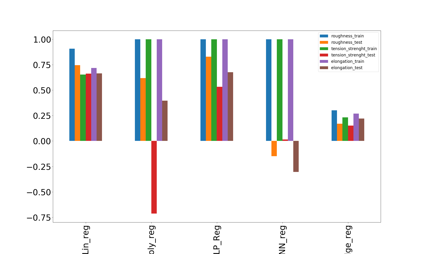
Conclusions

From the above comparisons, we can say that the polynomial regression, MLP regression and KNN regression gives the perfect accuracy of 1(100%) for the training set but the accuracy reduces (sometimes gone negative) drastically for the test set.
On the other hand for the linear regression, the test set accuracy is closer to that of the train set.
The other models (except linear regression and ridge) is kind of overfitting the train dataset. For the case of the ridge regression, the model is underfitting.
In future, I shall try to use the same dataset and explain how to use it for MTR.
That’s it for now, this is me Shibashis signing off for the day. Thanks for stopping by at mechGuru.com.
In case you want the complete code of both the parts, plesae visit my GitHub page.