Blog

In the Part-1 of the article we saw how to derive the cost function in case of liner regression for a simple problem:

Problem statement: want to predict the machining cost (let’s say Y) of a mechanical component, given the following inputs (let’s say X):

• Numbers_of_drilled_holes  (let’s say X1)
• Total_machined_volume_mm3 (let’s say X2)

We also have historical data:

And the cost function we derived is:

 Cost_function=(1/3)*[( 150 – {3*W_1 + 10*W_2+B})^2+( 500 – {5*W_1 + 50*W_2+B})^2+( 625 – {4*W_1 + 25*W_2+B})^2]………………..eq.7

In this article, we will see how the gradient descent algorithm find the local minima of the cost function, here the algorithm goes:

1. Calculate partial derivatives of the cost function(eq.7) with respect to all the independent variables (X’s):
   1. Partial derivative of the cost function with respect to W_1:

DW_1_CF=(1/3)*[{2*( 150 – 3*W_1 – 10*W_2-B)*(-3)} +{2*( 500 – 5*W_1 – 50*W_2-B)*(-5)}+{2*+( 625 – 4*W_1 – 25*W_2-B)*(-4)}]……eq.8

• Partial derivative of the cost function with respect to W_2:

DW_2_CF=(1/3)*[{2*( 150 – 3*W_1 – 10*W_2-B)*(-10)} +{2*( 500 – 5*W_1 – 50*W_2-B)*(-50)}+{2*+( 625 – 4*W_1 – 25*W_2-B)*(-25)}]……eq.9

• Partial derivative of the cost function with respect to B:

DB_CF=(1/3)*[{2*( 150 – 3*W_1 – 10*W_2-B)(-1)} +{2*( 500 – 5*W_1 – 50*W_2-B)(-1)}+{2*+( 625 – 4*W_1 – 25*W_2-B)(-1)}]……eq.10

• Put initial guesses of W_1, W_2 and B to the equations eq.8, 9, 10 and update the initial guesses as below:

W_1=W_1 – LR* DW_1_CF  ………………eq.11

W_2=W_2 – LR* DW_2_CF  ………………eq.12

B=B – LR* DB_CF  ………………eq.13

LR = Learning Rate (also called alpha)

• Keep repeating the above step-2 until :

Either,  LR* DW_1_CF, LR*DW_2_CF  and LR*DB_CF become very small (typically 0.001 is considered)

Or, Maximum numbers of iterations (called epochs) reached.

• The values of W_1, W_2 and B for which the conditions mentioned in the point 3 above is satisfied, are used for calculating the local minima using the eq.7

If it looks little too much of equations, don’t worry, we will jump to the code now, which will make the things much clear.

Lets load our data and visualize it:

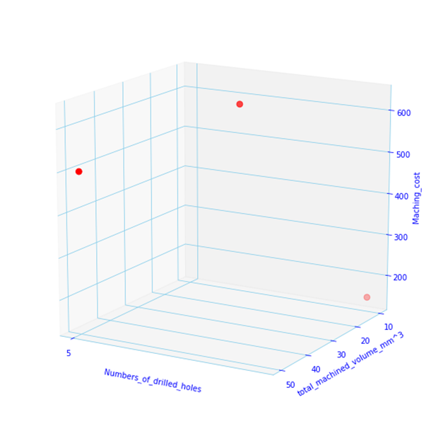
It looks little empty as we have very few data points, lets add some more:

And it looks much populated and interesting now:

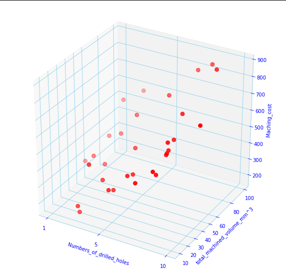
Since the numbers of data points have increased now (although its far less than real life examples), we need to generalize the cost function we derived in the eq.5 in the part-1 of this tutorial:

Cost_function = (1/n)*[( Y_1 – Y_pred_1)^2+( Y_2 – Y_pred_2)^2+( Y_3 – Y_pred_3)^2]………………..eq.5

Or, Cost_function=(1/n)*sum(Y-Y_pred)^2

Or, Cost_function(cf)=(1/n)*sum(Y-  X1*W1-X2*W2-B)^2…………………..eq.14

And the generalized form of the partial derivatives are:

DW_1_CF =(2/n)*sum[(Y-  X1*W1-X2*W2-B)(-X1)]……………………eq15

DW_2_CF =(2/n)*sum[(Y-  X1*W1-X2*W2-B)(-X2)]……………………eq16

DW_3_CF =(2/n)*sum[(Y-  X1*W1-X2*W2-B)(-1)]……………………eq17

Let’s see the code, finally:

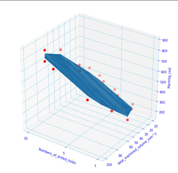
The blue surface is the prediction surface, And the red dots are the actual values of Machining_cost.

Let’s see from another view:

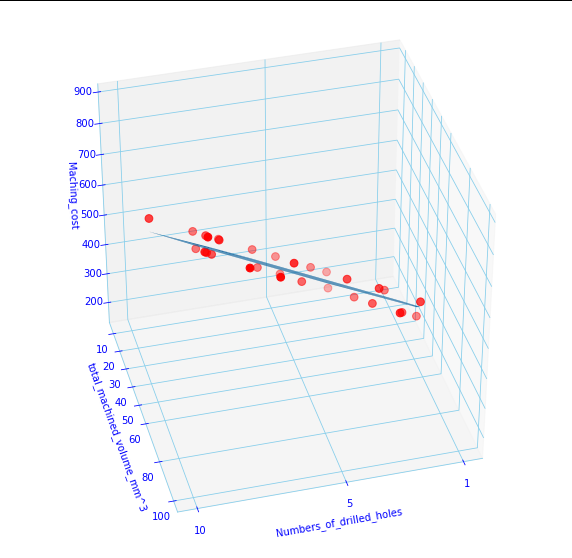
The code above will print the weights w1, w2 and b:

43.07234584367571 5.266662489230692 4.390903281111696

Observe the prediction plane is representing the actual machining cost reasonably well, but how could you say that statistically? And the answer lies in the cost function itself. use the w1,w2 and b  to find the cost (mean squared error or MSE) and if you take square root of MSE it is called RMSE. Another measure of the goodness of fit is r2 or r-squared :

and output:

root mean squared error: 32.736799131727366

r2 score: 0.9698647736277413

r2 is unit-less, it is saying that approximately 96% of the data fits the linear regression model which is quite good.

Let’s stop here, please let me know if you have any questions, suggestions. Thanks for reading.

Shibashis

Hi, I am Shibashis, a blogger by passion and an engineer by profession. I have written most of the articles for mechGuru.com. For more than a decades i am closely associated with the engineering design/manufacturing simulation technologies. I am a self taught code hobbyist, presently in love with Python (Open CV / ML / Data Science /AWS -3000+ lines, 400+ hrs. )