Blog

Gradient descent is a powerful algorithm used for optimizing many types of functions including the cost functions in data science

However, before going to the mathematics and python codes of it let first formulate a linear regression machine learning problem.

Problem statement: want to predict the machining cost (let’s say Y) of a mechanical component, given the following inputs (let’s say X):

• Numbers_of_drilled_holes  (let’s say X1)
• Total_machined_volume_mm3 (let’s say X2)

We also have historical data:

Linear regression

here we start with a general linear equation with X, Y and B (constant terms, also call bias term in ML lingo):

Y_pred= X*W+B………eq.1

W is a matrix of constants , also called weights. Also note all the terms of the above equation are matrix, so if you expand it:

                Y_pred_1 = 3*W_1 + 10*W_2+B

                Y_pred_2 = 5*W_1 + 50*W_2+B

So on…

Or, in general,

Y_pred_1 =X1_1*W_1 + X2_1*W_2+B…………..eq.2

Y_pred_2 =X1_2*W_1 + X2_2*W_2+B…………..eq.3

Y_pred_3 =X1_3*W_1 + X2_3*W_2+B…………..eq.4

And, for each of the rows, the deviation between the prediction and the actual or error is calculated simply as:

Error_1= Y_1 – Y_pred_1

and so on…

Further the quantify the total error the term Mean Squared Error (MSE) is used, and you guessed it right, the equation of it (also called Cost function in ML lingo):

Cost_function = (1/n)*[( Y_1 – Y_pred_1)^2+( Y_2 – Y_pred_2)^2+( Y_3 – Y_pred_3)^2]………………..eq.5

Where, n = number of rows in the historical data matrix

Now, if you plug the eq.2,3,4 in the eq.5:

Cost_function=(1/n)*[( Y_1 – {X1_1*W_1 + X2_1*W_2+B})^2+( Y_2 – {X1_2*W_1 + X2_2*W_2+B})^2+( Y_3 – {X1_3*W_1 + X2_3*W_2+B})^2]………………..eq.6

If we put the values of all X, Y and n:

Cost_function=(1/3)*[( 150 – {3*W_1 + 10*W_2+B})^2+( 500 – {5*W_1 + 50*W_2+B})^2+( 625 – {4*W_1 + 25*W_2+B})^2]………………..eq.7

Before going further, let’s visualize this cost function, however since it’s a multivariable function of more than two variable so for human being it will be difficult to visualize. So, for the sake of visualization, we will drop the B, and the below python code will plot the function:

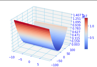
From the above plot, you can observe it’s a concave plane, hence, there exists a minimum. And you guessed it right, that’s where the tings will start getting interesting further.

However, we will stop here for this part and will go further in the next part of this article which will revolve around gradient descent algorithm.

Let’s summarize what we did so far in this part of the article,

 we started with general equations of Y_predict in the form of Y_predict=a1*X1+a2*X2+C. Since we are at linear regression, the general equation is linear in nature.

We then got the equation of MSE which we called cost function and we visualized it.

See you in the Part-2 of this article.

Shibashis

Hi, I am Shibashis, a blogger by passion and an engineer by profession. I have written most of the articles for mechGuru.com. For more than a decades i am closely associated with the engineering design/manufacturing simulation technologies. I am a self taught code hobbyist, presently in love with Python (Open CV / ML / Data Science /AWS -3000+ lines, 400+ hrs. )